General Function Checklist
Annotation Track Operators
Note: Be sure to look at the user guide pages linked here. Skim them to make sure that the topics they cover are represented here (if not add points here as needed). Read enough to ensure that the instructions and explanations are clear, and the page has accurate information and generally appears up-to-date.
See Users Guide pages:
single track - output an annotation track
- Open the A_thaliana_Jun_2009 genome.
- Go to this region: Chr1:2,992,975-3,012,448
- Load the TAIR10 mRNA track via the Available Data section (IGB Quickload > TAIR10 other annotations).
- Select the Annotation tab at the bottom of IGB, and look for the Operations box.
single track - copy
- Select the ( - ) track and select Copy, hit Go.
- Select the ( + ) track, select Copy, hit Go.
- Combine the ( - ) and ( + ) tracks into one using the +/- checkbox.
- Select the +/- track, select Copy, hit Go.
- In the Annotation tab, use Select All, and under Strand, check the Arrow option (to make visual verification easier).
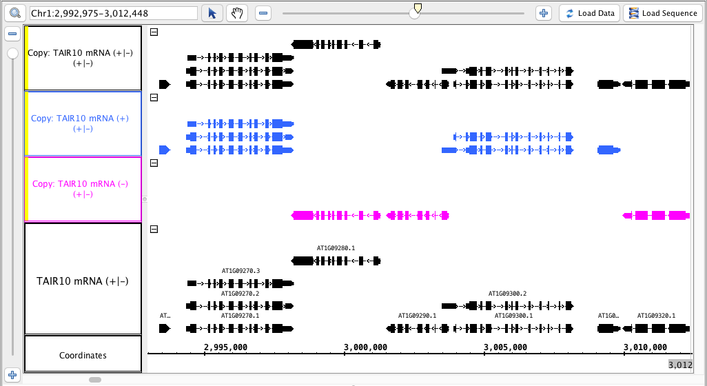
- The tracks produced match the image above (color matching is optional).
- Mac
- Linux
- Windows
- The track names for the new tracks indicate which track they were made from AND which strand ( -, + or +/- )
- Mac
- Linux
- Windows
- The tracks made from only one strand have only the annotations from that strand.
- Mac
- Linux
- Windows
- The track made from both strands has annotations from both strands.
- Mac
- Linux
- Windows
single track - not, summary
- Delete the tracks you just created.
- Split the TAIR10 mRNA track back into separate - and + tracks.
- Select the ( - ) track, select Not, hit Go.
- Select the ( + ) track, select Not, hit Go.
- Recombine the - and + tracks.
- Select the ( +/- ) track, select Not, hit Go.
- Repeat all of the above for the Summary operation.
- Color the tracks that were made from the ( - ) strand pink and the ( + ) blue for visual verification.
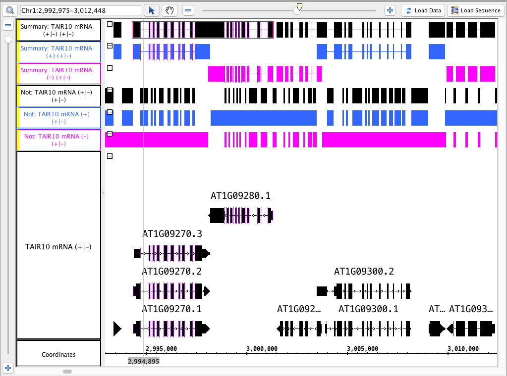
- Your IGB looks like the image above.
- Mac
- Linux
- Windows
multi track - output an annotation track
- Using the combined (+/-) TAIR10 mRNA track, run the Summary operation and the Not operation.
- Hide the original track and highlight the two newly created tracks (hold shift and click each one) --Select the Not track first.
- Perform each of the multi-track operations:
- A not B
- B not A
- Intersection
- Union
Xor

- Your IGB looks like the image above.
- Mac
- Linux
- Windows
- Track labels include the names of the operation and the input tracks.
- Mac
- Linux
- Windows
- Each track is identical to the "Not" track, or identical to the "Summary" track, or completely solid, as appropriate.
- Mac
- Linux
- Windows
- Delete the tracks you just created.
- Using the split ( - ) and ( + ) TAIR10 mRNA track, perform each of the multi-track operations:
- A not B
- B not A
- Intersection
- Union
- Xor
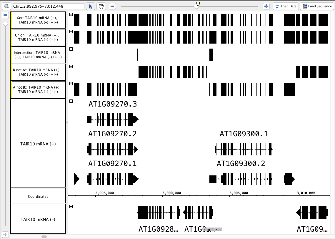
- Your IGB looks like the image above (Particularly notice the area around the zoom stripe, it highlights the difference between Union and Xor.)
- Mac
- Linux
- Windows
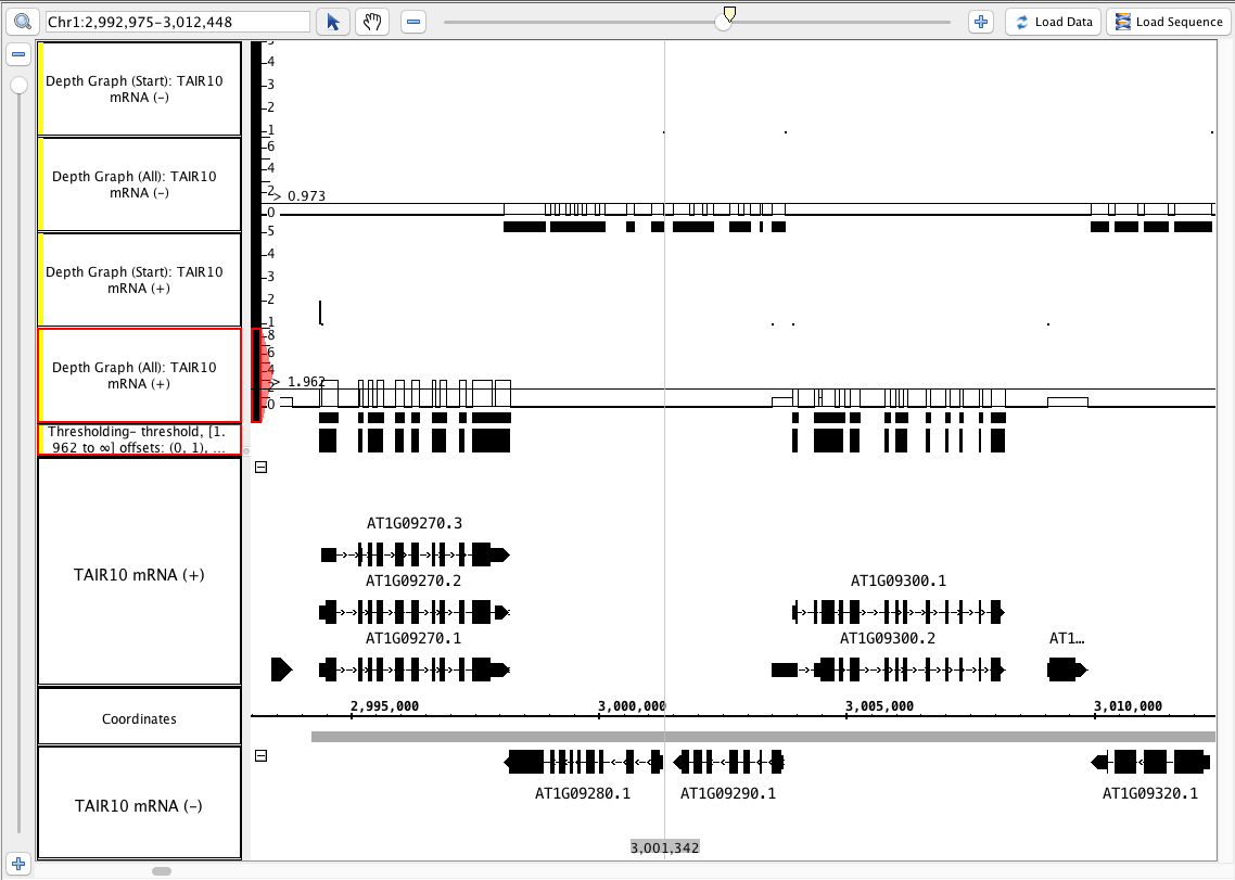
single track - output a graph track from a bed file
- Use the + and - tracks separately to run each of these operations (this produces 4 graph tracks).
- depth (all) (single track)
- depth (start) (single track)
- Repeat this by selecting both the - and the + track at the same time (hold shift) and selecting the above single track operations.
- The results of step 1 and 2 above are identical.
- Mac
- Linux
- Windows
- Select one of the depth (all) graphs.
- In the Graph panel, choose Thresholding...
- Set Visibility to On.
- Slide the By Value slider back and forth.
- The little blocks appear and disappear as the line touches the graph.
- Mac
- Linux
- Windows
- The values in the graph track correspond to counts of annotations that cover each location.
- Mac
- Linux
- Windows
Click Make Track.
- The new track looks correct based on the By Value threshold that you set.
- Mac
- Linux
- Windows
- The new track has an appropriate label that indicates what threshold was used to create it.
- Mac
- Linux
- Windows
- Your IGB looks similar to the image above (notice that the depth (start) graphs have data in a 1-base-wide area at the start of the annotations, and where there is only 1 annotation, the graph has a height of 1).
- Mac
- Linux
- Windows
single track - output a graph track from a bam file (part 1)
Go to this region: Chr1:2,998,442-3,001,453
From the RNA-Seq Quickload in the Available Data section, add the RNA-Seq / Pollen SRP022162 / Reads / Pollen alignments file.
Click Load Data, then Load Sequence.
Select the Pollen alignments track and run the following single track operations:
- Select Find Junctions, enter 5, hit go.
- Select Find Junctions, enter 10, hit go.
- Select Find Junctions (tophat), enter 5, hit go.
- Select Find Junctions (tophat), enter 10, hit go.

- Your IGB looks like the image above (*Read the junctions user guide page for more details).
- Mac
- Linux
- Windows
Right click blank space in any of the tracks, then click Optimize Track Height.
- The sizes of the blocks for the Find Junctions tracks match the value you entered; the Find Junctions (tophat) results will not all have the same block size.
- Mac
- Linux
- Windows
- The count above each junction is equal to the number of reads that matched that gap.
- Mac
- Linux
- Windows
- Find someplace where the matching Find Junctions operation using value 5 and value 10 have different scores. Identify the read(s) that matches that junction, and where where one side of the read is between 5 and 10 bases.
- Mac
- Linux
- Windows
- Right-click on the Pollen alignments track and select Track Operations > Copy.
- Right-click on the copied track and look at the options listed within the Track Operations.

- The above options are listed for the copied Pollen alignments track under Track Operations.
- Mac
- Linux
- Windows
single track - output a graph track from a bam file (part 2)
- Open the H_Sapiens_Dec_2013 genome.
- Add the smoke testing Quickload using the Available Data section: http://igbquickload.org/smokeTestingQuickload/
- Add the Bam (binary alignment with index) track to IGB.
- Go to this region: chr1:2,180,492-2,180,751
- Click Load Data, then click Load Sequence.
- Select the Bam (binary alignment with index) track and do the following single track operations:
- depth (all) (single track)
- depth (start) (single track)
Mismatch Graph
Mismatch Pileup Graph
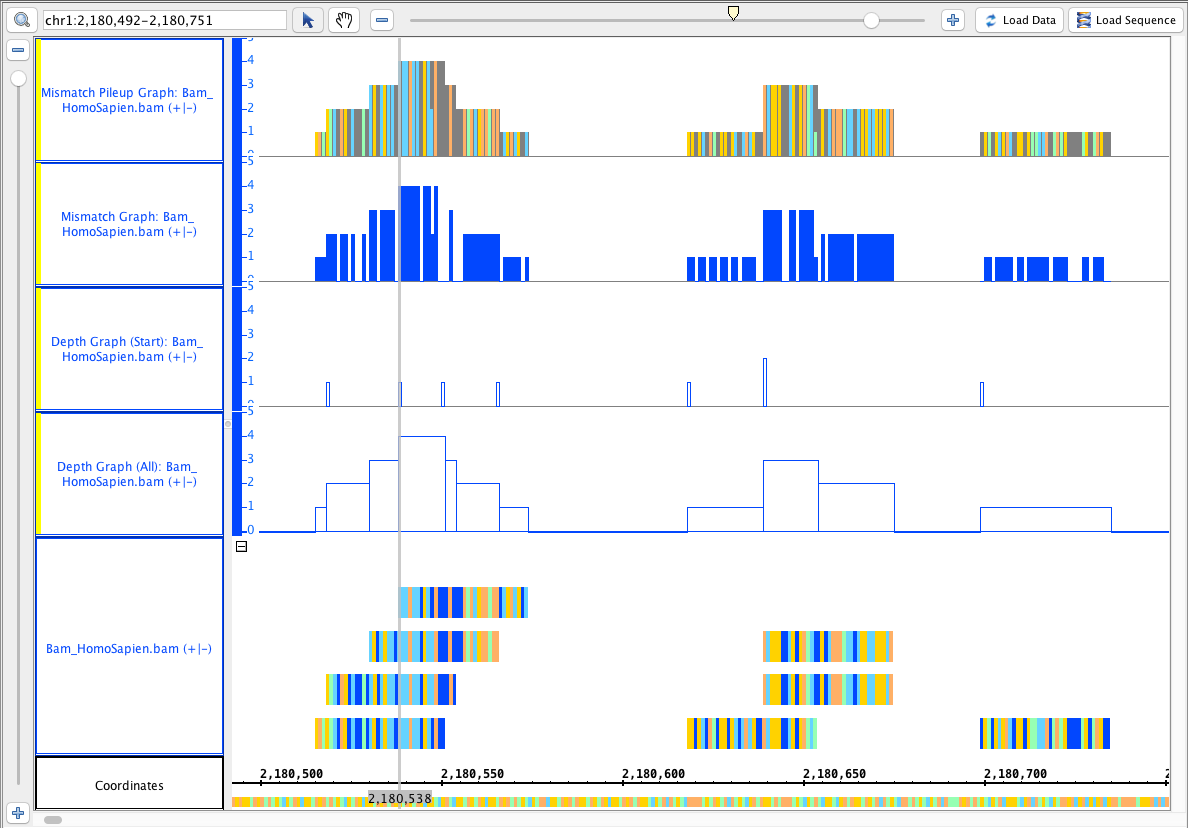
- Your IGB looks like the image above.
- Mac
- Linux
- Windows
- Zoom out to the following coordinates: chr1:2,180,361-2,180,883
- Click Load Data (do not load sequence). Load data a second time if needed, but not a third.
- The sequence loaded as needed after a max of two time clicking Load Data.
- Mac
- Linux
- Windows
Go to this region: chr1:3,785,135-3,785,276
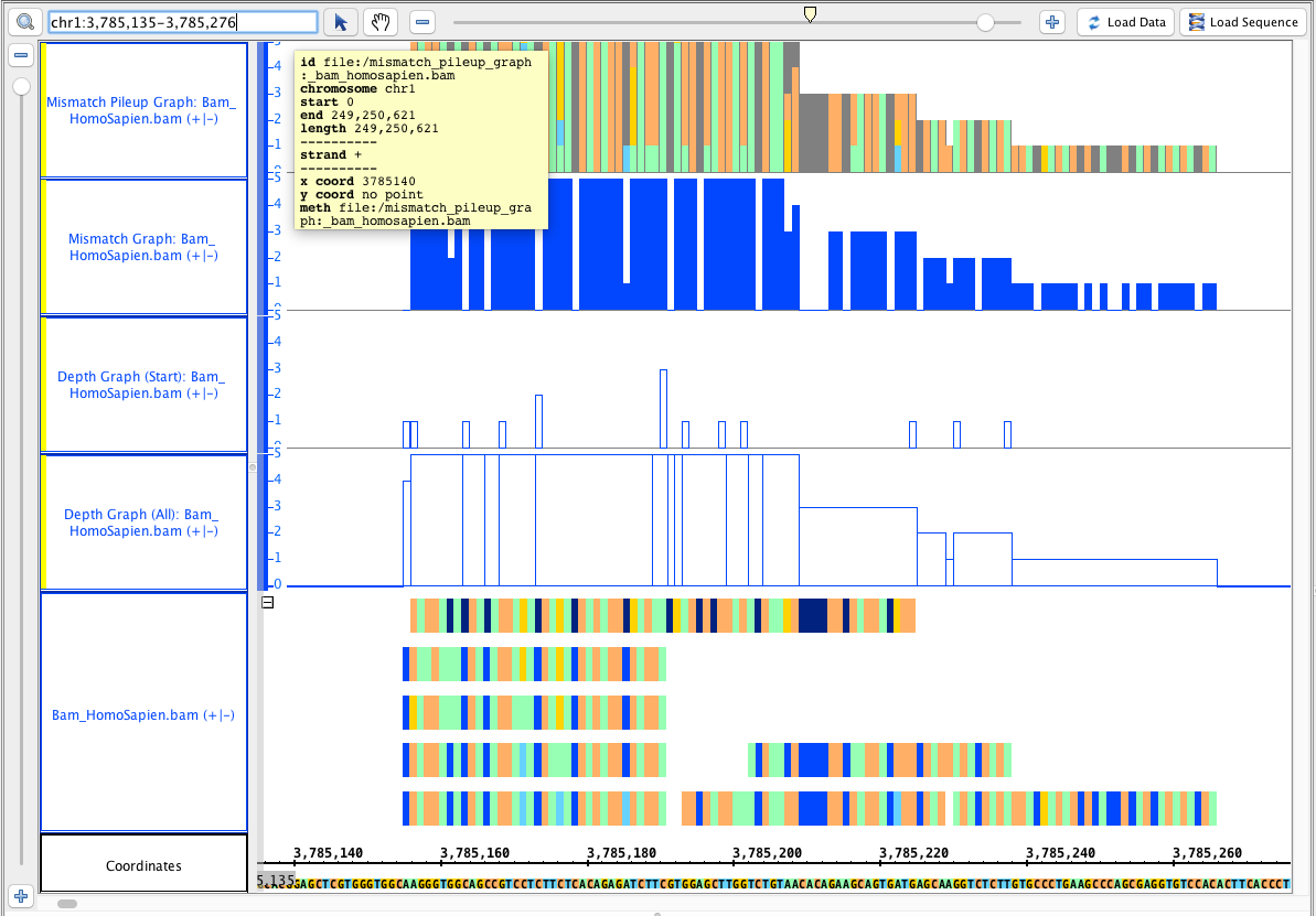
- Your IGB looks like the image above.
- Mac
- Linux
- Windows
Users Guide
Review the users guide pages.
Each page has accurate information and generally appears up-to-date.
- Mac
- Linux
- Windows