Introduction

IGB contains several functions that allow you to create all new annotation and graph tracks from existing tracks.

These functions can help identify new genes, new splicing variants, and help expose biologically meaningful aspects of your data. You can save the new tracks as BED format files, which you can re-open later in IGB and share with others.

There are two types of track functions

• Single-track functions that apply to one track only
• Multi-track functions that apply to two or more tracks

Single track functions

To access single-track functions

• Select a track
• Click Annotations sub-panel
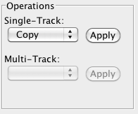
• Choose a function from the Operations sub-panel

Annotation tab

OR

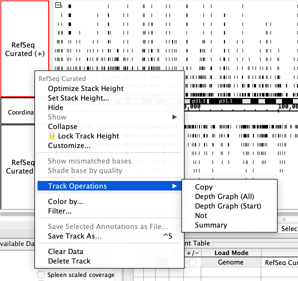
• Right-click a track label
• Choose Track Operations

Right-click menu

Not

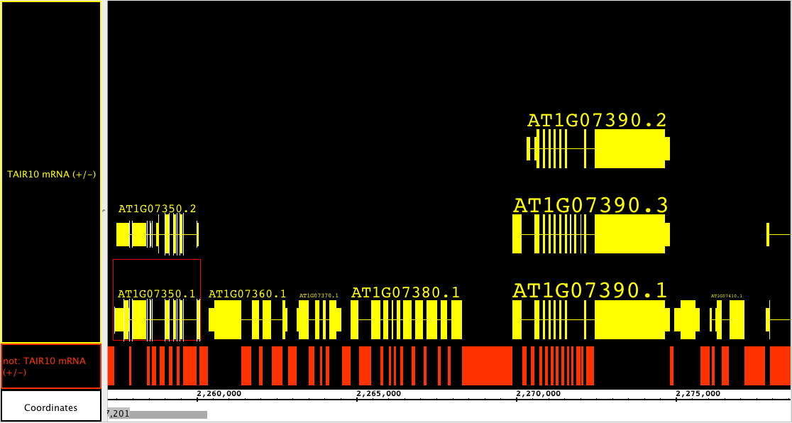
Not creates a new track with annotations representing empty regions from the selected track.

Copy

This function simply produces a copy of the original, with no changes to the annotations.

Multi-track functions

To access multi-track functions

By performing the functions below, IGB can provide new annotation tracks showing a uniquely specified/analyzed data set. This can be merged annotations, or annotations of areas where only one or the other track have data This powerful set of functions can help discover new features of all types within the data. For instance, selecting a RNA-seq experimental track followed by a reference sequence track and choosing A not B will show you all of the places where there are RNA reads that do not align to the annotated genome; all of the annotations in the newly created track could represent retained introns, new exons, new exon-intron boundaries, and even whole new genes.

These actions are specific to the tracks and strands that you selected, i.e. you can select just the + strand or just the - strand of a data set. This can be used to your advantage; for instance, if you want to know where on the chromosome there are annotations that overlap on the forward and reverse strands, then choose the + strand and the - strand and use the Intersect operation.

Another place where performing track comparisons is useful is when you are comparing treatments of samples versus controls. Depending on the function chosen, the new tracks will show differences or similarities, or even regions left completely unaffected. This can even be used with thresholding tracks created from graphs. By comparing 2 different tracks with different threshold settings, these operations can show you what is different between the two cases. To capture the graph thresholds in a track, see Applying thresholds to graphs.

To combine tracks:

• Select two or more tracks by clicking and SHIFT-clicking the track labels. The first track selected is designated 'A' and the second track is 'B'.
• Right-click a selected track label and choose Track Operations. 

Choose one of the options listed.  The effects of each option is described below.

Intersect

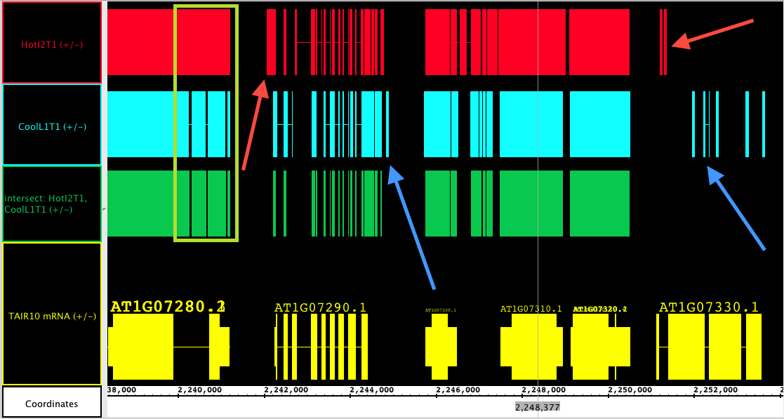
Yields only the overlapping portions of A and B. This is good for looking at similarities between tracks. Although not quantitative, this is a good way to find out what similar elements are present or not. The picture below shows the intersection  track, in green, of two .bam files (shown collapsed) and their reference sequence (also collapsed). Here you can see that they generally have the same genes expressed, even though they may be expressed at different levels. The red arrows are pointing out where ONLY the treatment track has reads; blue arrows show only control reads. The green box highlights the fact that if either track has gaps (such as introns) they will show in the intersection track.

Union

Yields all bases that are in either A OR B

A not B, B not A

A not B and B not A tracks show the part of track 'A' that does not overlap with track 'B' and vice versa. These tools are incredibly powerful for finding differences between two tracks. You can find differences due to treatments, between expressed sequences (RNA-seq) and annotated tracks (reference sequences) or between different versions of data sets. There are many other applications as well.

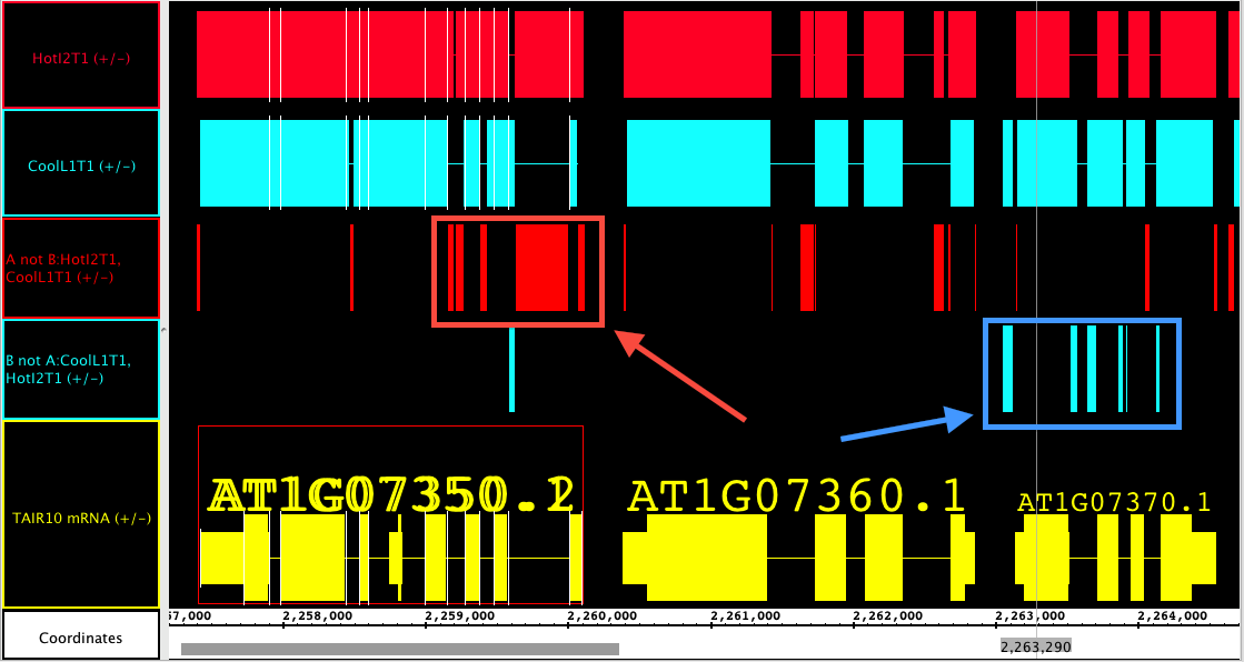
To use these functions in IGB, select track 'A' first, and then track 'B'. The new track label indicates the function and the order of the track selection, i.e. in the image below the track label "A not B:HotI2T1, Cool L1T1(+/-)"  indicates A not B was used to generate the track and that HotI2 is 'A' and CoolL1 is 'B'. In this image, the A not B track shows all of the instances where there is data present in HotI2 that are not matched in CoolL1 (red box, red arrow). Meanwhile, the B not A track shows CoolL1 data that is not present in HotI2 blue box, blue arrow).

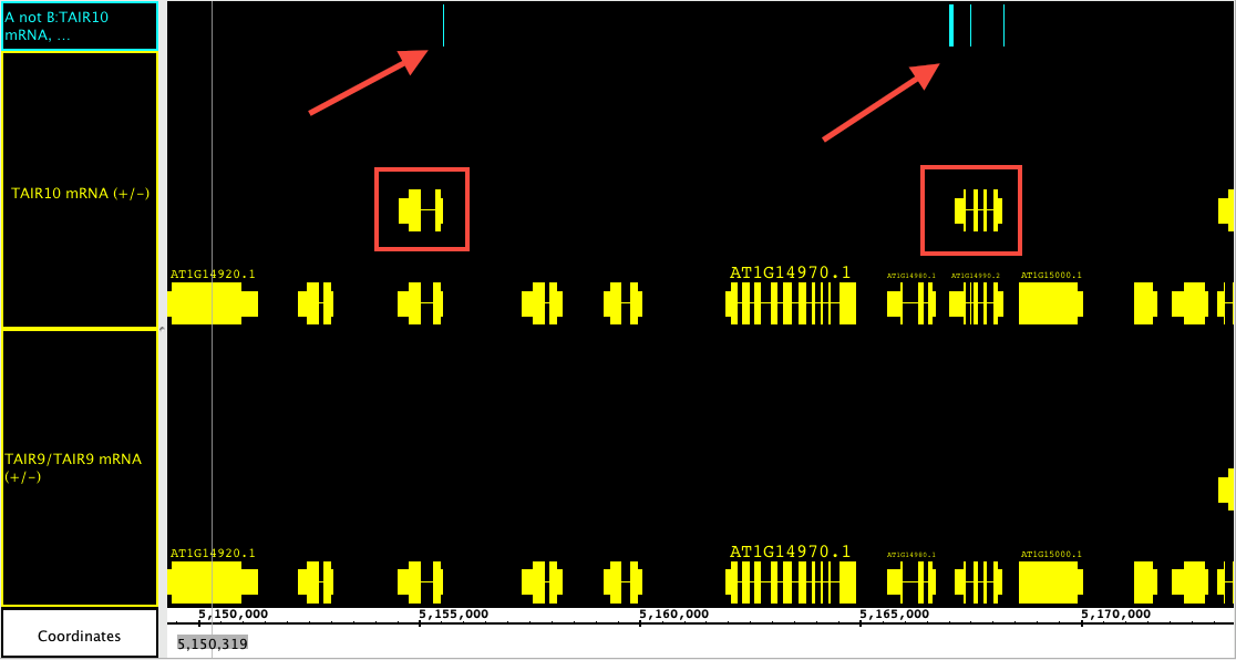
In this track, we compare TAIR10 annotations to older TAIR9 annotations to find differences. You can see that there are 2 new splice variants included in this region, but that they do not look very different from the original by a quick glance. the A not B track identifies exactly where they are different.

XOR

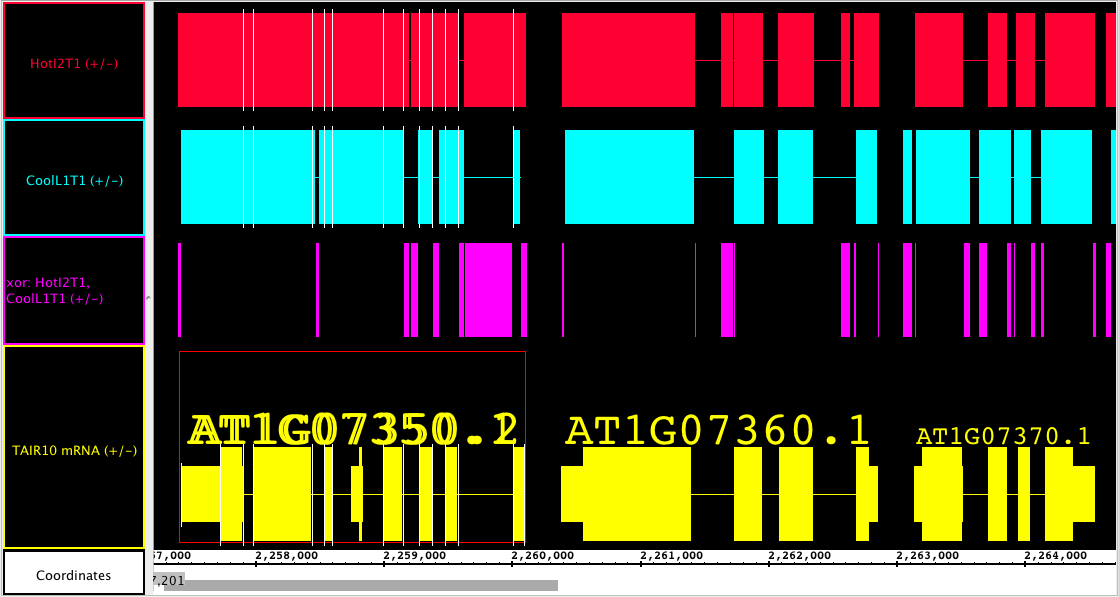
XOR tracks shows the union of the material that is in A or B but not both; this is like a summary track of both A not B and B not A. Order of track selection is irrelevant here. While this track summarizes the differences into one track, you cannot determine which of the original tracks contains the difference, but it makes and excellent way to skim across data looking for general regions of difference.