Graphs can be created by right-clicking on a track's label and highlighting Track Operations. A list of graphs and other track operations compatible with the track are displayed and may be selected to create a child track. The track operations that create graphs are:

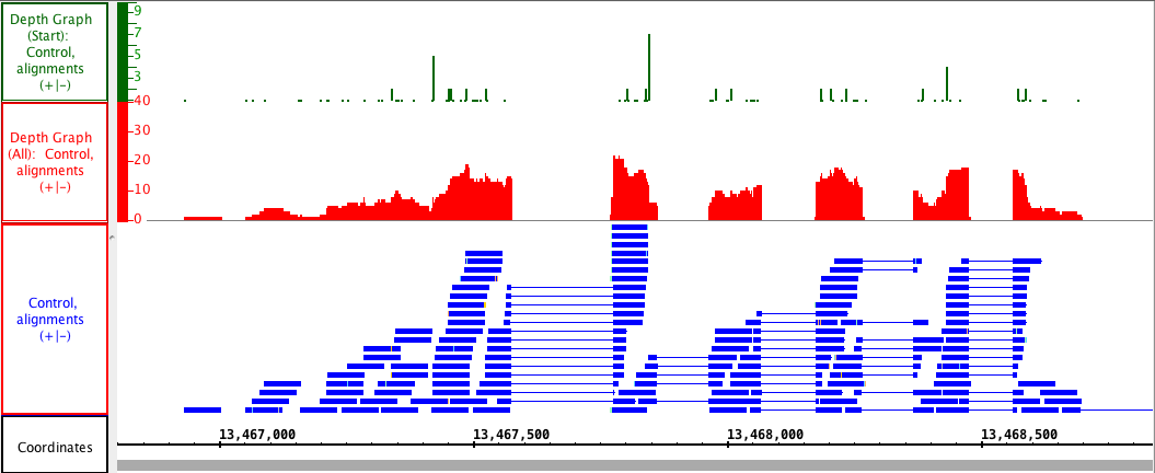
• Depth Graph (All)
• Depth Graph (Start)
• Mismatch Graph
• Mismatch Pileup Graph

After these graphs are created, click Load Data to load graphs for regions that have not yet been loaded. Graph tracks may be saved as .wig formatted files.

The Depth Graph feature works for all annotations but is most useful in combination with a Mismatch Graph. This allows you to see how many reads are present at each nucleotide position (Depth Graph) and where mismatches occur as compared to the genomic sequence file (Mismatch Graph).

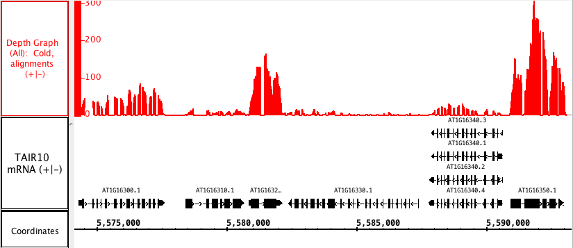
Depth Graph (All)

Depth Graph (All) allows you to generate an overview of the relative density of annotation coverage across an entire chromosome (this is also known as a coverage graph).  This feature dynamically graphs the number of annotations in a track that are present at each nucleotide across the genomic sequence. When you are completely zoomed in, and each pixel represents a single nucleotide base, the graph shows actual values for the number of reads aligned at that genomic location. Using the Select tool to hover over a particular point in the graph will open a tooltip with the actual number of reads at that point.

Right-click on the track's label and choose Track Operations > Depth Graph (All).

The picture below shows a fully expanded BAM file, showing the difficulty of seeing any details. The second picture shows just the depth graph (*BAM *track is 'hidden').

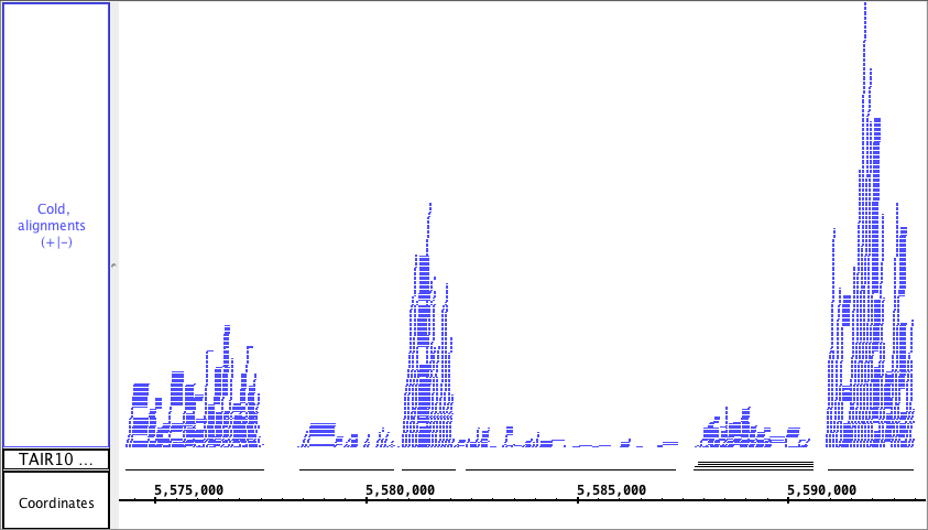
Depth Graph (Start)

Depth Graph (Start) only graphs the first nucleotide of each read. This is most useful when assessing coverage bias in RNA-Seq or other high-throughput sequencing experiments. Often some regions are better represented than others, thanks to PCR amplification bias or other artifacts.

Mismatch Graph

The Mismatch Graph is specific to short read alignment files, such as BAM.  The graph shows only the number of mismatched nucleotides across all reads at a specific genomic location, which can be very helpful in the detection of allelic variation, SNP identification and also error checking. Right click in the label to access the menu; choose Track Operations > Mismatch Graph. This function requires that the genomic sequence be loaded; if it is not loaded, IGB will load the sequence for you.

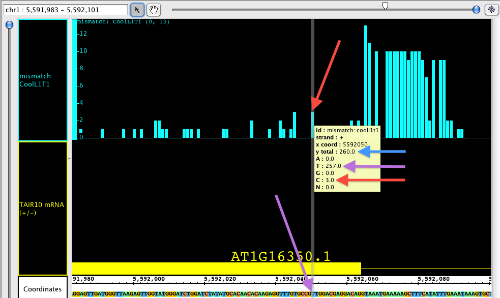
If you hover the Select tool (arrow cursor) over an individual bar of the graph, you will get a tool tip showing the total number of reads, and then the number of reads broken down by nucleotide. In the picture below, you can see that the total number of reads at the specified position is 260 (blue arrow). Of those reads, 257 at at 'T', which you can see is the matching nucleotide (purple arrows). 3 of those reads contain a 'G' instead; since G is a mismatch, the graph shows a bar with height of 3 (red arrows).

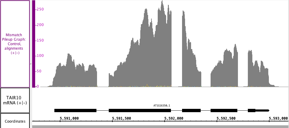
Mismatch Pileup Graph

In the Mismatch Pileup, you have the Depth Graph portion represented as a dark gray graph, with the Mismatch Graph overlayed in the matching nucleotide colors. The colors show which and how many of each nucleotide(s) are present at each mismatch position. The Mismatch Pileup graph, like the Mismatch Graph, is also specific to short read alignment files, such as BAM. Right click in the label to access the menu; choose Track Operations > Mismatch Pileup Graph. This function requires that the genomic sequence be loaded; if it is not loaded, IGB will load the sequence for you. 

In the image below, you can see the gray portion is a Depth Graph, but you can also see the mismatched nucleotides (very small numbers in this section), which are color coded by G, A, T and C.