Introduction
Graphs contain numerical data associated with base pair positions along the chromosome sequence axis, such as sets of scores or chromosome copy numbers at specific positions. IGB allows you to visualize such graph data and compare it with RefSeq and other annotations.
Examples of suitable data include:
- Files generated from Affymetrix software tools, such as the Expression Console, CNAT, GCOS, or ExACT.
- Expression values from genome tiling arrays.
- Density of ESTs across chromosomes
- GC content along chromosomes
- Measures of conservation between two genomes
There are two basic types of graphs:
- Position graphs associate scores with single genomic positions.
- Interval graphs associate scores with ranges of genomic positions.
Here is a very simple example of several interval graphs:
IGB will recognize whether the graph is a position or interval graph and will display it accordingly.
The child pages explain how to use IGB to examine your graph data:
- Compare graph and annotation data in the same region.
- Adjust graphs to highlight features
- Fine-tune graph scaling to improve visibility
- Use thresholding to transform graph data into annotation-like format, in order to examine it further using other tools in IGB.
Loading graph files
Graph files are loaded in the same way as annotation data files. To open graph files in any of the supported formats:
- Follow the procedures in Loading Data.
IGB can display graphs in several file formats, developed at Affymetrix or elsewhere. All file names must include the file name extension, such as ".sgr". Compressed files must include the graph type extension AND the compression extension, such as "mygraph.sgr.zip". For the list of all file formats IGB supports, see File Formats. Graph files may be in the following formats:
.bar |
Generated from tiling arrays by TAS (Tiling Analysis Software.) |
.chp |
Binary files generated by Affymetrix software. These files contain data on scores for probe sets. There are multiple variations on this file format. IGB can read some, but not all of these formats. |
.egr |
Files containing data for scored intervals. |
.sgr |
Sequence graph files that show base coordinate scores. These files are generated by CNAT (the Affymetrix Chromosome Copy Number Analysis Tool software). |
.gr |
A simple text format containing two columns of numbers separated by a single space or tab. The first number is the base position; the second number is the score. |
.useq |
A binary format used for both graphs and annotations. Supported in IGB 6.2. For more information about it, see: http://useq.sourceforge.net. |
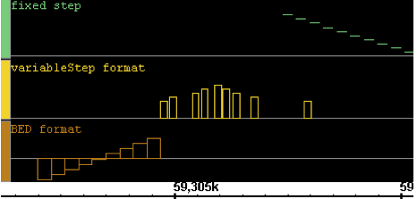
.wig |
Wiggle format. A text format developed for use in the UCSC genome browser. All three sub-formats of wiggle graph are supported by IGB: "fixedStep", "variableStep" and "BED". |
Note: Set Species and Genome Version before loading graph files, as you would for annotation files. Graph files in some formats (notably .gr) do not contain information about which genomes and chromosomes they correspond to. These may be loaded and displayed alongside annotations on any chromosome, but the data may have no meaning if compared to the a chromosome it was not designed for. i.e., to use a .gr file, you must first load the proper organism, genome AND chromosome prior to loading the .gr file
Hiding and deleting graphs
Hide graphs to remove them from the display without deleting them from memory. Right click on the graph track label and choose Hide from the menu, just as you would do for annotation tracks. Note: floating graphs must be 'docked' by deselecting Floating before they can be hidden. Hidden graphs can be restored by right clicking in ANY track and using the Show function. To hide one or more tracks:
- Select the tracks (or use the Select All button in the Graph Adjuster panel to select all graph tracks).
- Right click and select Hide.
Delete graphs to permanently remove them from the viewer and from memory. To delete one or more graphs:
- Select the graph or graphs.
- Click the Delete button.
Alternatively, just click the trashcan icon next to the graph file name in the Data Access panel, as you would for an annotation track.