Hiding and deleting graphs
Hide graphs to remove them from the display without deleting them from memory. Hidden graphs can be restored later. Delete graphs to permanently remove them from the viewer and from memory.
For a graph attached to a tier, you can hide it in the same way you hide an annotation tier. Right-click on the label tier and select Hide from the menu. Floating graphs must be attached to a tier before they can be hidden.
To delete one or more tiers:
- Select the tier label.
- Right click and select "Delete Selected Tiers".
To delete one or more graphs:
- Select the graph or graphs.
- Open the Graph Adjuster tab. Click the Delete button.
To delete all graphs currently displayed on this chromosome:
- Choose File menu > Clear graphs.
To delete all graphs currently displayed on all chromosomes:
- Choose the Whole Genome view
- Choose File menu > Clear graphs.
Advanced graph manipulations
Controls for the graph features below can be found in the Advanced section of the Graph Adjuster tab.

Graph labeling
You can modify the labels for graphs that are currently selected by checking checkbox options in the Advanced portion of the Graph Adjuster panel.
- Show or hide the Y Axis scale
- Show or hide the identifying Label of the graph source (typically the same as the name of the graph file)
An example graph showing both options turned on is shown below:

...
Floating graphs
An attached graph appears in its own track, like other annotation types. A floating graph is drawn on top of other tracks with a transparent background. Since a floating graph is not in a track, it has no track handle. Instead, use the graph handle to select the graph, or to drag it to a new location. The graph handle is the colored bar to the left-hand side of the graph.
Controls for floating or attaching a graph can be found in the Advanced section of the Graph Adjuster tab.
To attach a graph into its own regular graph track:
- Click the colored bar at the left side of the graph (the graph handle) to select it, then deselect the Floating checkbox.
To detach a graph from its track and let it float:
- Click the colored bar at the left side of the graph (the graph handle) to select it, then select the Floating checkbox.
You can set default preferences so that graphs load either initially floating or attached as a track. See Setting graph preferences.
Transforming to a non-linear scale
By default, all graphs display in linear scale. If you wish to scale the data in a non-linear way:
...
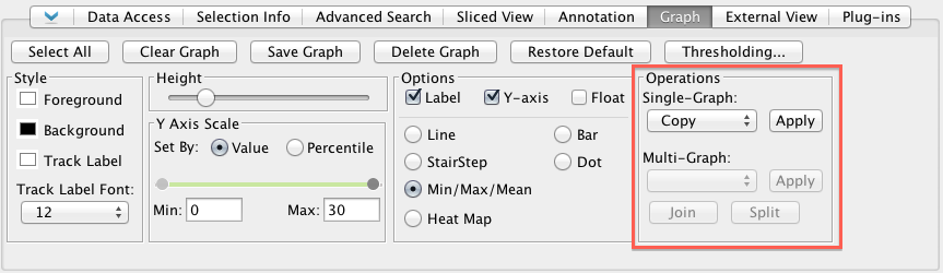
Operations - making new graphs from old ones
IGB supports multiple types of graph manipulations via the Operations section of the Graph tab. To perform a graph operation:
- Select the graph (or graphs) by clicking the corresponding track label. SHIFT-click to select more than one .)graph.
- Click Select the Graph Adjuster tab.
- Select the type of transformation you would like to perform from the pull-down menu labeled Transformation in the Advanced section.
- Click GO
IGB duplicates your graph in a new track and applies the selected scale to the new graph. Your original graph is not deleted. Note that one of the choices of scale is Copy, which makes a copy of the graph without re-scaling it. That can be useful if you want to explore the effects of showing one graph in two graph styles at the same time.
Duplicating graphs
You may want to duplicate a graph to experiment with different graph adjustments without losing adjustments that you have already made.
To duplicate a graph:
- Click the colored bar at the left end of a graph to select it.
- Click the Graph Adjuster tab. In the Advanced section, under the label Transformation select Copy and click Go.operation you wish to perform
Note that single-graph operations operate on single graph tracks. Multi-graph operations operate on two or more tracks.
The result will appear in a new track, labeled with the operation used to create it. When you load new data, the track containing the result of the operation will update.
Tip: Save the result to a file by right-clicking the track and select Save As. Only data for the current chromosome will be saved. (This may change in future releases of IGB.)
Joining and splitting graphs
It is possible to join two or more graphs into a single annotation track. The two graphs will then have a single track tier label and can be moved and adjusted as a group.
To join multiple graphs, select them, then press the Join button in the Advanced portion of the Graph Adjuster panel. To separate graphs that were earlier joined together in this way, select them and press the Split button.
When the tier is in the expanded state, the multiple graphs are shown in separate non-overlapping bands:

If the tier is collapsed, all graphs are shown in the same, overlapping band:

When joined graphs are collapsed, any opaque regions of the top graph will hide corresponding features of the lower graph or graphs.
Joining graphs into a single annotation track can be very useful for expression data from multiple experiments. Here, data from several experiments at different times during the development of an organism are shown together in a single track, and it is easy to see that expression of genes is being regulated over time.
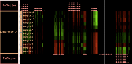
By selecting the single tier label, here labeled "Experiment A", you can easily set the graph style and data range for all these graphs to be identical.
Graph arithmetic
You may need to compare the relative differences in expression levels between two graphs that represent data that occupy the identical genomic position on the chromosome. For example, a graph of cancerous cells will show what's turned on or off when compared to a graph of normal cells. Results that show significantly more or less activity than a control graph for the same region may indicate an area of interest.
Arithmetically combining two graphs may make the differences and correlations easier to see.
To arithmetically combine two graphs:
- Shift-click the bar at the left end of each graph to select the graph. The graph you click first is A, the graph you click second is B.
- Use one of the four Combine buttons in the Advanced portion of the Graph Adjuster tab labeled A+B, A-B, A*B, and A/B.
- Alternatively, right-click the bar at the left end of either graph and choose Combine Graphs, then choose one of the following:
- Create Sum Graph (A+B)
- Create Difference Graph (A-B)
- Create Product Graph (A*B)
- Create Ratio Graph (A/B)
 Graphs that are joined into one track share a track label. Operations performed on the joined graph apply to each of the joined graphs.
To join graphs:
- Select two or more graphs by SHIFT-clicking their track labels
- Select Graph tab
- Click the Join button (under Operations)
To separate joined graphs:
- Select the joined graph by clicking its track label
- Select Graph tab
- Click the Split button (under Operations)
Tip: Use the Y Axis Scale settings to put joined graphs onto the same scale. Click the "collapse" tool (upper left of joined graph track) to overlay and compare the joined graphs. Or set their style to Heat Map to view multiple experimental samples in the same track. For example, the following image shows data from a developmental time course highlighting expression changes over time.